Model-based Reinforcement Learning

27 Sep 2017

In this post, we will cover the basics of model-based reinforcement learning. After some terminology, we jump into a discussion of using optimal control for trajectory optimization. We first understand the theory assuming we have a model of the dynamics and then discuss various approaches for actually learning a model. We end with a discussion and derivation of using optimal control with learned time varying linear models, which is a state-of-the-art algorithm that can be used in robotics to quickly solve real world tasks! This also serves to introduce important concepts, such as using KL divergence to constrain policy updates and using dual gradient descent to solve constrained optimization problems.

Intro

We will first address the case where the transition dynamics are known. That is, we have a function \(f\) that tells us what the next state (or the distribution over the next state) is given the current state and action.

\[f(s_t, a_t) = s_{t+1}\]

In model-free reinforcement learning, we make no attempt to use or learn the transition function. We just try our best to learn a policy that produces the best possible action given an input state. Intuitively, it should seem that knowing exactly how our actions and states leads to future states gives us more information and allows us to choose better actions. Indeed, this is often the case!

Model-based approaches can be useful in practice because we often do know the dynamics or have the ability to construct a model of the dynamics. For example, in simulated environments, games, and simple real-world systems, we have a very good idea of how the system behaves in response to actions. It’s natural to want to use this additional information.

Terminology

Open-Loop vs Closed-Loop

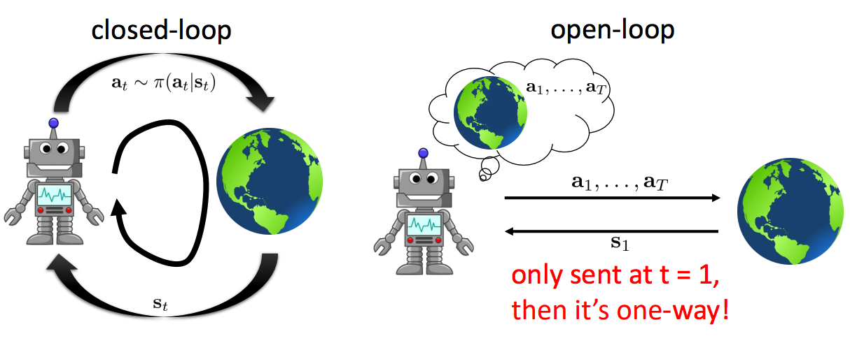
An open-loop system is one that provides no feedback. We are given the initial state and must immediately output a sequence of actions. This corresponds to solving an optimization problem to find the sequence of actions that maximizes the expected reward:

\[a_1, a_2, \ldots , a_n = \arg\max_{a_1, a_2, \ldots, a_n} \mathbb{E} [\sum_t r(s_t, a_t)|a_1, a_2, \ldots, a_n]\]

In contrast, a closed-loop system does provide feedback. We’re given a state and asked to produce an action. Once we produce the action, the world is updated and returns to us the next state, and the loop repeats!

It should make intuitive sense that we can perform better under a closed-loop system: we get feedback for our actions. As an example, suppose we want a robot to take actions to enter a building and retrieve an object. It’s hard to plan an exact sequence of actions to take if the robot is outside the building and does not know what is inside the building. It’s much easier to enter the building, observe what’s in the building, and then take actions from there.

To add to this intuition, we can generally do a better job of choosing action \(a_k\) conditioned on the observations \(o_1, o_2, \ldots, o_{k - 1}\) rather than choosing action \(a_k\) with no prior knowledge.

Optimal Control

Optimal control gives us solutions to these problems where we know the dynamics. We’ll change our notation to be consistent with the optimal control literature. In general the problem we wish to solve is the following:

\[\min_{u_1, \ldots, u_t} \sum_{t= 1}^T c(x_t, u_t) \text{ s.t. } x_t = f(x_{t-1}, u_{t-1}) \\ \begin{align*} &u_t \text{ is the action at time step t} \\ &x_t \text{ is the state at time step t} \\ &f \text{ is the transition function} \\ &c \text{ is the cost function (negative reward of RL problem)} \\ \end{align*}\]

Note that we have a minimization problem since we are expressing everything in terms of costs rather than rewards. Equivalently, we can pose this as an unconstrained optimization problem by rewriting the states in terms of our actions.

\[\min_{u_1, \ldots, u_t} c(x_1, u_1) + c(f(x_1, u_1), u_2) + \ldots + c(f(\ldots), u_t)\]

We could try to use calculus to solve this system via differentiation and gradient descent. However, this is often not a good idea in practice because there is high sensitivity to the first action, so the gradients are ill-conditioned.

For the coming discussion, it might be useful to keep a real world example in mind. The task could be to insert a block into a shape sorting cube. In this case, the state consists of the joints of the robot (and possibly a visual observation), the action corresponds to torques applied to the joints, and the cost could be the distance from the cube to its desired target.

Linear-quadratic regulator (LQR)

It turns out that we can obtain the optimal solution under some simplifying assumptions. In particular, if we assume the dynamics are linear and the costs are quadratic in the states and actions, we can solve for the optimal sequence of states and actions. This should be a pleasant surprise! In model-free reinforcement learning, we generally have no such theoretical guarantees.

Here’s a high level description of the algorithm:

1. We work from the end \((t = T)\) to the beginning \((t = 1)\). This is because \(u_T\) shows up exactly once in the optimization objective, so we can solve for it (via setting the partial derivative to 0) in terms of \(x_T\). We can then write the last cost term entirely in terms of \(x_T\), which we don’t yet know (the state at time step \(T\) depends on all our earlier actions).

2. At time step \(t = T - 1\), the action \(u_{T-1}\) affects both the \((T - 1)\)st cost term and the next state, \(x_T\). Since we know exactly the dynamics and the cost of \(x_T\), we can solve for \(u_{T-1}\) in terms of \(x_{T-1}\).

3. Continuing to go backwards through time, we notice that each action affects the cost function at the step and the next state. This means the optimal actions are linear functions of the state at every time step! When we reach \(t = 1\), we have a policy or controller (something that spits out an action given the state) at every time step.

4. But we know the very first state \(x_1\)! This means we can determine the optimal action \(u_1\) with our controller. This then gives us \(x_2\) via the dynamics model. We continue with this forward pass to compute the optimal actions and states to minimize the quadratic cost.

More formally, let our transition dynamics and cost be:

\[x_{t+1} = f(x_t, u_t) = \boldsymbol{F_t} \begin{bmatrix} x_t \\ u_t \end{bmatrix} + f_t\] \[c(x_t, u_t) = \frac{1}{2} \begin{bmatrix} x_t \\ u_t \end{bmatrix}^T \boldsymbol{C} \begin{bmatrix} x_t \\ u_t \end{bmatrix} + \begin{bmatrix} x_t \\ u_t \end{bmatrix}^T c^t\]

We define the quantity \(Q(x_t, u_t)\) to be the cost-to-go or the sum of the remaining costs (from time \(t\) to time \(T\)):

\[Q(x_t, u_t) = \sum_{i=t}^T c(x_i, u_i) \text{ s.t. } x_t = f(x_{t-1}, u_{t-1})\]

and define the value function as \(V(x_t) = \min_{u_t} Q(x_t, u_t)\). This is consistent with reinforcment learning definitions for value functions and Q values. The full derivation is left as a guided exercise.

Exercise: It’s recommended to start by writing \(\boldsymbol{C}\) as a \(2 \times 2\) block matrix reflecting how it hits \(x_t\) and \(u_t\).

• Show the \(u_T\) that minimizes \(Q(x_T, u_T)\) is linear in \(x_T\). That is, \(u_t = \arg\min_{u_t} Q(x_t, u_t) = K_t x_t + k_t\) where \(K_t\) is a matrix you will define. Again, this is nice because we have a policy: given a particular state, we have a simple function that returns to us the optimal action to take.
• Show that \(V(x_T)\) is quadratic in \(x_T\).
• Verify that \(Q(x_t, u_t) = c(x_t, u_t) + V(f(x_t, u_t))\). Compute \(Q(x_{T - 1}, u_{T - 1})\) and then show that \(u_{T - 1}\) that minimizes \(Q(x_{T - 1}, u_{T - 1})\) is again linear in \(x_{T - 1}\).

We actually get the same solution if we assume that our transition function has some Gaussian noise, independent of the state or action.

iLQR

LQR is great and all because we obtain the optimal solution, but what happens if we have more complicated dynamics or cost functions? Enter iterative LQR.

The high-level view of iLQR is very similar to that of Newton’s method: we start with some initial trajectory (sequence of states and actions), and iteratively update the trajectory by approximating the complicated dynamics and cost with simple, tractable functions and then optimizing over the simpler functions.

More specifically, given some complicated \(f(x_t, u_t)\) and \(c(x_t, u_t)\) and trajectory \((\hat{x}_t, \hat{u}_t)_{t=1}^N\), we can use Taylor expansions to form linear dynamics and a quadratic cost that are accurate in the region close to the current trajectory. The dynamics and cost are expressed in terms of differences with the current trajectory, \(x_t - \hat{x}_t\) and \(u_t - \hat{u}_t\)

Then using LQR, we perform a backwards pass giving us a controller

\(u_t - \hat{u}_t = K_t (x_t - \hat{x}_t) + k_t\).

at every time step (note how the controller is now expressed in terms of differences with our original actions and states). To get an updated trajectory, we run the forward pass using our controller and the true nonlinear dynamics of our system. We then repeat this entire process of function approximation and optimization with the new generated trajectory.

One practical consideration is that because our approximation is local, it may not hold if a new trajectory is far away from the original \(\hat{x}_t\) and \(\hat{u}_t\). To avoid the problem of moving into a region where the dynamics are very off, we can define our controller as follows:

\[u_t = K_t (x_t - \hat{x}_t) + \alpha k_t + \hat{u}_t\]

where \(\alpha \in [0, 1]\) and perform a line search on \(\alpha\) to minimize the cost. Notice that \(\alpha = 0\) results in no update to the trajectory while \(\alpha = 1\) is the best update if we had true linear dynamics and quadratic cost, so optimizing on \(\alpha\) can be though of as interpolating between the old trajectory and the new trajectory.

As a side note, if we keep everything else in the algorithm the same but use a quadratic approximation to the dynamics instead of a linear one, we are performing exactly Newton’s method. In the context of optimal control, this method is called differential dynamic programming (DDP). It’s more expensive but potentially more accurate than iLQR. iLQR generally works well enough in practice.

One final note is that if we parametrize the iLQR policy as a Gaussian:

\[\mathcal{N}(K_t (x_t - \hat{x}_t) + k_t + \hat{u}_t, \sigma_t)\]

we get something called a time-varying linear model. The special structure of these controllers means that they can be learned very quickly and have very high representational power (to get results on real robots). More on this later.

Unknown Dynamics

Up to now, we’ve assumed that we’ve been given a model. What happens if we want to do model-based reinforcement learning but don’t have a model? We try to learn the model from data.

Exercise: How would you learn a dynamics model from data? What can you do to increase the likelihood that your dynamics model is accurate in regions of state space that you care about?

Here are various algorithms, roughly in increasing order of sophisication.

1

1. We run a policy (potentially random) to collect state transition data \(D = \{(s, a, s')_i \}\).
2. We then train a function \(f\) to approximate the dynamics such that \(f(s, a) \approx s'\). For example, \(f\) is a neural network that minimizes mean squared error.
3. We train a policy with the dynamics model. Train in a loose sense, such as by running iLQR.

Analysis: This is simple to implement. The problem is that the dynamics model may not be relevant or accurate in the states that we care about, as the data collected is from some other policy.

2

1. We run a policy (potentially random) to collect state transition data \(D = \{(s, a, s')_i \}\).
2. We then train a function \(f\) such that \(f(s, a) \approx s'\).
3. We train a policy with the dynamics model.
4. We execute actions from the policy generated in step 3 and add the transitions to \(D\). Go to step 2.

Analysis: This fixes the problem described above in a manner similar to how DAgger improves performance. Note that this is treating the problem as an open-loop system, so we can still do better!

3

1. We run a policy (potentially random) to collect state transition data \(D = \{(s, a, s')_i \}\).
2. We then train a function \(f\) such that \(f(s, a) \approx s'\).
3. We train a policy with the dynamics model.
4. We generate actions by iteratively replanning. We execute the first planned action, add the trajectory to \(D\), and then replan to choose the next action.
5. After some number of time steps, we go back to step 2.

Analysis: This method of replanning after every action is known as model-predictive control (MPC). The idea is that by constantly replanning, we can fix the policy if our original plan goes awry. This agrees with the notion that closed-loop systems work better than open-loop systems earlier. The more we replan, the less accurate the plans need to be. This approach can be computationally expensive. Note that this approach even works when plans are generated randomly, as described in this paper!

4

1. We run a policy (potentially random) to collect state transition data \(D = \{(s, a, s')_i \}\).
2. We then train a function \(f\) such that \(f(s, a) \approx s'\).
3. We initialize with some policy, then update the policy by computing the gradient of the cost with respect to the policy parameters. This can be done since we know the gradients with respect to the transition function and the policy. We are backpropagating through time.
4. Append trajectories generated by the policy to the dataset, then go back to step 2.

Analysis: This one has a different feel from the earlier approaches because it tries to train a policy (possibly a neural network). The problem is that gradients may vanish or explode, similar to problems encountered while training recurrent neural networks.

Parametrizing the Model

One component we have yet to discuss is what function we use to parametrize the dynamics. One type of model is a Gaussian process which is data-efficient, but struggles with non-smooth dynamics and is slow to train when the dataset is large. Learning to Control a Low-Cost Manipulator using Data-Efficient Reinforcement Learning is an example of a paper that uses backpropagation through a Gaussian process model.

Another choice is a neural network. In a neural network, optimizing mean squared error loss corresponds to fitting a Gaussian to maximize \(p(s' \vert s, a)\). Neural networks are expressive and deal well with large amounts of data, but can struggle with low amounts of data.

These are two of the more common choices for function approximators when learning dynamics, but other alternatives are possible.

Local Models vs. Global Models

There’s one more detail on models we need to address. Note that we need a sufficently good model to converge to a satisfactory solution. Otherwise, the policy tends to exploit the model in regions where the model is overly optimistic.

One way to build a model to build a global model, a single function that models the dynamics in all of state space. The problem is that it can be difficult to encapsulate all the information in one single function, especially if we have reason to believe the dynamics are different in different parts of state space. For example, robotics tasks with contacts have extermely complicated dynamics.

A potentially more tractable approach is to build accurate local models. Notice that in the discussion on optimal control, we actually didn’t need a global model! Instead all we needed are the local gradients: \(\frac{df}{dx_t}\) and \(\frac{df}{du_t}\).

One concern with local models though is that they become inaccurate as soon as our policy updates, since they are by definition, local. We’ll soon see some ways to counteract this problem. In general, the tradeoff in time complexity is that local models are easier to fit, but need to be thrown away whenever the policy updates because they are only accurate for trajectories collected under the old policy.

Before diving into doing model-based RL with local models, one other idea worth mentioning is that global models are beneficial in that they generally maintain some sort of consistency in state space i.e. states close to each other generally have similar dynamics. We can approximiately get this same desirable behavior by using a global model as a prior in training local models. This is called Bayesian linear regression and can help reduce sample complexity.

Optimal Control with Local Models

We will now tie together all these ideas into a very powerful one that can train robots to solve tasks quickly in the real world! Many of these ideas show up up in the paper Learning Contact Rich Manipulation Skills with Guided Policy Search. This approach boils down to a three step loop:

1. Run controller (that we get from optimal control) on robot to collect trajectories.
2. Fit dynamics model to collected trajectories.
3. Update policy with new dynamics model.

Note the similarity to vanilla iLQR. The difference is that we collect trajectories to fit local models rather than using linearizations of a global model of the dynamics. We’ll now describe the procedure in greater detail.

Running the controller

Recall that running iLQR produces a controller:

\[u_t = K_t (x_t - \hat{x}_t) + k_t + \hat{u}_t\]

The controller we use matters a lot because we are trying to fit local dynamics, in the region of the controller. We can’t just run some arbitrary controller.

Our choice of controller is a Gaussian with the same mean as the iLQR controller: \(K_t (x_t - \hat{x}_t) + k_t + \hat{u}_t\) and variance \(\sigma_t\). This allows us to correct for drifts that occur because of errors in the dynamics. It’s important to not choose a deterministic controller because we need variability in our collected trajectories to be able to better fit local dynamics (you can’t fit a line about a single point). A particularly clever choice of the variance of the Gaussian is:

\[\sigma_t = Q_{u_t, u_t}^{-1}\]

where \(Q_{u_t, u_t}\) denotes the part of the quadratic cost function associated with the actions \(u_t\) (recall our decomposition of the cost matrix). Intuitively, a high value means that the cost is sensitive to changes in a particular action, so setting the inverse as the convariance means we want to be more careful and reduce the variance of the action.

More formally, it turns out the controller \(\mathcal{N}(K_t (x_t - \hat{x}_t) + k_t, Q_{u_t, u_t}^{-1})\) optimizes the original cost function minus the conditional entropy of the action given the state:

\[\min \sum_{t=1}^T \mathbb{E}_{(x_t, u_t)} [c(x_t, u_t) - H(u_t | x_t)]\]

(if you are unfamiliar with entropy, it’s intuitively speaking a measure of the randomness of a distribution. Higher entropies correspond to probability distributions that are closer to uniform, which means that we are less certain about the outcome.) Since our maximization is over the conditional entropy of the action, this leads to the controller maximizing the randomness in the action while minimizing the original cost. This is exactly the type of controller we want!

Fitting dynamics

We fit a local model at every time step:

\[p(x_{t+1} \vert x_t, u_t) = \mathcal{N}(A_t x_t + B_t u_t + c, \sigma)\]

This can be done via simple linear regression to the transitions collected by the controller \(\{x_t, u_t, x_{t+1}\}_i\). As described above, we can do better via Bayesian linear regression by introducing a global prior on the dynamics.

Improving the controller

We want to improve our controller, but to not change the controller so much that it lead to us moving to regions where our model is inaccurate. To do this, we limit the KL divergence between the controller and updated controller. KL divergence is defined as:

\[D_{KL} (p(x) \vert \vert q(x)) = \sum_{x} p(x) \log{\frac{p(x)}{q(x)}} = \mathbb{E}_p [\log p(x) - \log q(x)]\]

(intuitively, KL divergences measures the dissimilarity between two different probability distrbutions. Placing a bound on how big the KL divergence can be limits how much we can change our policy)

We want to compute the KL divergence between our new policy’s trajectory distribution \(p(\tau)\) and the old one \(\bar{p}(\tau)\). This is written as \(D_{KL}(p(\tau) \vert \vert \bar{p}(\tau))\). We can express both trajectory distributions in terms of the initial state distribution, policy, and dynamics.

\[p(\tau) = p(x_1) \prod_{t = 1}^T p(u_t \vert x_t) p(x_{t+1} \vert x_t, u_t)\] \[\bar{p}(\tau) = p(x_1) \prod_{t = 1}^T \bar{p}(u_t \vert x_t) p(x_{t+1} \vert x_t, u_t)\]

Notice that the only thing that changes is the policy, since we assume the dynamics are unchanged. This means that taking the difference of the logarithms of the trajectory distributions cancels out a bunch of terms.

\(\begin{align*} D_{KL}(p(\tau) \vert \vert \bar{p}(\tau)) &= \mathbb{E}_{p(\tau)} [\log p(\tau) - \log \bar{p}(\tau)] \\ &= \mathbb{E}_{p(\tau)} [\sum_{t = 1}^T \log p(u_t \vert x_t) - \log \bar{p}(u_t \vert x_t)] \\ &= \mathbb\sum_{t = 1}^T \mathbb{E}_{p(x_t, u_t)} [\log p(u_t \vert x_t) - \log \bar{p}(u_t \vert x_t)] \\ &= \mathbb\sum_{t = 1}^T \mathbb{E}_{p(x_t, u_t)} [- \log \bar{p}(u_t \vert x_t)] + \mathbb{E}_{p(x_t)p(u_t|x_t)} [\log p(u_t \vert x_t)] \\ &= \mathbb\sum_{t = 1}^T \mathbb{E}_{p(x_t, u_t)} [c(x_t, u_t) - H(p(u_t \vert x_t))] \end{align*}\) where we apply linearity of expectation and use the definition of conditional entropy. We substitute \(c(x_t, u_t) = - \log \bar{p}(u_t \vert x_t)\).

This optimization problem can be solved by the iLQR controller! \(\bar{p}(u_t \vert x_t)\) doesn’t depend on the current controller and can be thought of as a cost function: it takes in state and action pairs and outputs a scalar. The iLQR controller with the special variance term optimizes a cost function minus an entropy term.

This idea of bounding the KL divergence in a policy update is used in other areas of reinforcement learning (such as model-free algorithms) and is a convenient tool to keep in mind.

The one remaining issue is that we want the KL divergence to be in our objective, whereas it’s natural to express it as a constraint: \(D_{KL}(p(\tau) \vert \vert \bar{p}(\tau)) < \epsilon\). We’ll take a brief digression into dual gradient descent to address this issue.

Dual Gradient Descent

In optimization, we often want to solve constrained problems.

\[\min_x f(x) \text{ s.t. } C(x) = 0\]

To make the problem unconstrained, we form the Lagrangian:

\[\min_x \max_\lambda L(x, \lambda) = \min_x \max_\lambda f(x) + \lambda C(x)\]

Note that \(x\) necessarily has to satisfy the constraint \(C(x) = 0\); otherwise, the inner max can force an unbounded value \(+ \infty\). We can consider the dual problem:

\[\max_\lambda \min_x L(x, \lambda)\]

Any value for the dual provides a lower bound on the solution to the original (primal) problem. Under strong duality conditions, the optimal values are equal. Dual Gradient Descent (or ascent) aims to solve this problem via an iterative algorithm. We define \(g(\lambda) = \min_x L(x, \lambda)\).

1. Start with some initial \(\lambda\).
2. Solve for \(x^* \leftarrow \arg\min_x L(x, \lambda)\).
3. Compute \(\frac{dg}{d \lambda}\). Take a gradient step \(\lambda \leftarrow \lambda + \alpha \frac{dg}{d \lambda}\)
4. Repeat steps 2 and 3 until convergence.

One way step 2 can be solved is by setting the gradient to 0. In the case of trajectory optimization, it corresponds to iLQR.

In step 3, computing \(\frac{dg}{d \lambda}\) is easy given \(x^*\), which is a function of \(\lambda\):

\[\frac{dg}{d \lambda} = \frac{d}{d \lambda} L(x^*(\lambda), \lambda) = \frac{dL}{d x^*} \frac{d x^*}{d \lambda} + \frac{dL}{d \lambda} = \frac{dL}{d \lambda}\]

since \(\frac{dL}{d x^*} = 0\). \(\frac{dg}{d \lambda} = \frac{dL}{d \lambda} = C(x)\) has the nice interpretation of being how much we are violating the constraint. The more we violate the constraint, the more we increase the value of \(\lambda\), which penalizes violating the constraint. I’ve created a notebook to illustrate Dual Gradient Descent in action.

Improving the controller (continued)

We now apply the dual gradient descent algorithm to perform a constrained update on the controller.

\[\min_{p} \mathbb\sum_{t = 1}^T \mathbb{E}_{p(x_t, u_t)} c(x_t, u_t) \text{ s.t. } D_{KL}(p(\tau) \vert \vert \bar{p}(\tau)) \leq \epsilon\]

In the first step of DGD, for a fixed \(\lambda\), we try to solve:

\[\begin{align*} p^* &= \arg \min_{p} \mathcal{L}(p, \lambda) \\ &= \arg \min_{p} \mathbb\sum_{t = 1}^T \mathbb{E}_{p(x_t, u_t)} [c(x_t, u_t) - \lambda \log \bar{p}(u_t \vert x_t) - \lambda H(p(u_t \vert x_t)] - \lambda \epsilon \\ &= \arg \min_{p} \mathbb\sum_{t = 1}^T \mathbb{E}_{p(x_t, u_t)} [\frac{1}{\lambda} c(x_t, u_t) - \log \bar{p}(u_t \vert x_t) - H(p(u_t \vert x_t)] - \epsilon \\ \end{align*}\]

Then, defining \(\bar{c}(t) = \frac{1}{\lambda} c(x_t, u_t) - \log \bar{p}(u_t \vert x_t)\) as the cost function, we can run iLQR to get the optimal \(p^*(u_t \vert x_t)\). Note this new cost function has the nice interpretation of penalizing actions that were not likely under the old policy.

Exercise: Why does this interpretation make sense?

In the second step of DGD, we update \(\lambda\):

\[\lambda \leftarrow \lambda + \alpha (D_{KL}(p(\tau) \vert \vert \bar{p}(\tau)) - \epsilon)\]

This also has a nice intuitive interpretation: if we are violating the KL divergence constraint, then we increase \(\lambda\), which means we decrease the weight of the original cost function and put greater emphasis on matching the actions taken by the old policy.

Then we iterate until convergence! This concludes step 3, and we return to collecting more trajectories with this updated policy. Again, Learning Contact-Rich Manipulation Skills with Guided Policy Search is a paper that uses this approach for robotic manipulation.

Conclusion

We’ve discussed the foundations of model-based RL. In fact, we’re most of the way there to being able to understand guided policy search! A future post on GPS will hopefully appear soon.

Thanks Noah Golmant for reading an earlier version of this post.

Most of this post is me distilling information from Professor Sergey Levine’s lectures and slides in CS294-Deep Reinforcement Learning.

If you have any questions, feedback, or suggestions at all, please leave a comment.

Last updated: 1/6/18 (edits to clarity and typos)